SurfZar Deep-Dive: Differential Geometry Probing (Gaussian & Mean Curvature), Implicit CSG & Watertight 3D Printing

In our earlier articles on iSurfer and SurfZar, we explored how WebGL2 fragment shaders ray-trace implicit algebraic surfaces $f(x, y, z) = 0$ in real time.

However, a true mathematical laboratory needs more than visual rendering:

1. Differential Geometry Inspection (SurfacePointProbe.ts): When a mathematician or student clicks any point on a 3D surface, what is the exact Tangent Plane, Gaussian Curvature ($K$), Mean Curvature ($H$), and local surface classification (elliptic, hyperbolic, parabolic, planar, or singularity)?
2. Constructive Solid Geometry (CSG) & Homotopy Morphing (MeshExporter.ts): How do we combine two algebraic equations $f_1(\mathbf{p}) = 0$ and $f_2(\mathbf{p}) = 0$ via boolean operations, smooth organic blends, or continuous topological homotopies?
3. Watertight 3D Printing: How do you turn an infinitely thin mathematical zero-set $f(x, y, z) = 0$ clipped by a bounding sphere into a solid, manifold STL/OBJ/GLB sculpture that a 3D printer slicer (Bambu Studio, PrusaSlicer) can actually print?

Here is how those three subsystems work under the hood in SurfZar.

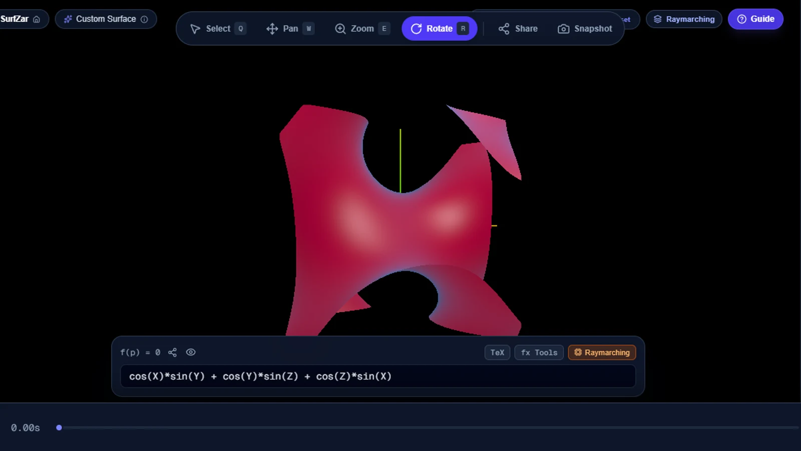
Click to zoomSurfZar Studio — Inspecting and morphing high-genus algebraic manifolds

---

1. Computing Gaussian ($K$) & Mean ($H$) Curvature Without Surface Parameterization#

In classical differential geometry textbooks, curvature is usually taught using a parametric surface patch $\mathbf{r}(u, v)$ via the First and Second Fundamental Forms.

But for an implicit algebraic surface $f(x, y, z) = 0$ (such as the Barth Sextic or Gyroid), no global $(u, v)$ parameterization exists!

In src/lib/SurfacePointProbe.ts (computeDifferentialGeometryAtPoint), when a user clicks on the 3D canvas, we cast a picking ray $\mathbf{r}(t) = \mathbf{o} + t\mathbf{d}$, refine the intersection point $\mathbf{p}^* = (x, y, z)$ via Newton-Bisection, and compute the gradient vector $\nabla f$ and the symmetric $3 \times 3$ Hessian matrix $\mathbf{H}_f$ using central finite-difference stencils:

$\nabla f = \begin{bmatrix} f_x \\ f_y \\ f_z \end{bmatrix}, \quad \mathbf{H}_f = \begin{bmatrix} f_{xx} & f_{xy} & f_{xz} \\ f_{xy} & f_{yy} & f_{yz} \\ f_{xz} & f_{yz} & f_{zz} \end{bmatrix}$

The Implicit Curvature Determinants#

Using the classical adjugate Hessian / bordered Hessian formulas for implicit surfaces, we compute the Gaussian Curvature $K = \kappa_1 \kappa_2$ and Mean Curvature $H = \frac{1}{2}(\kappa_1 + \kappa_2)$ directly from $\nabla f$ and $\mathbf{H}_f$ in $\mathbb{R}^3$:

$K = -\frac{1}{\|\nabla f\|^4} \det \begin{bmatrix} f_{xx} & f_{xy} & f_{xz} & f_x \\ f_{xy} & f_{yy} & f_{yz} & f_y \\ f_{xz} & f_{yz} & f_{zz} & f_z \\ f_x & f_y & f_z & 0 \end{bmatrix}$

$H = -\frac{\nabla f^\top \mathbf{H}_f \nabla f - \|\nabla f\|^2 \operatorname{tr}(\mathbf{H}_f)}{2 \|\nabla f\|^3}$

From $(K, H, \|\nabla f\|)$, SurfacePointProbe.ts automatically classifies the local differential geometry at the probed point:

And from the unit normal $\mathbf{n} = \nabla f / \|\nabla f\|$, it formats the exact Tangent Plane equation at $\mathbf{p}^*$:

$n_x(X - x_0) + n_y(Y - y_0) + n_z(Z - z_0) = 0$

---

2. Implicit CSG Booleans, Smooth Blending & Homotopy Continuation#

Because implicit surfaces represent geometry as scalar fields $f: \mathbb{R}^3 \to \mathbb{R}$, buildCompositeEvalFn (src/lib/MeshExporter.ts) can combine a primary equation $f_1(\mathbf{p})$ and secondary equation $f_2(\mathbf{p})$ into a composite scalar field $F(\mathbf{p})$ both in the GLSL shader and in the mesh exporter:

1. Exact Ricci CSG Booleans:
   • Union ($\mathcal{S}_1 \cup \mathcal{S}_2$): $F(\mathbf{p}) = \min(f_1(\mathbf{p}),\, f_2(\mathbf{p}))$
   • Intersection ($\mathcal{S}_1 \cap \mathcal{S}_2$): $F(\mathbf{p}) = \max(f_1(\mathbf{p}),\, f_2(\mathbf{p}))$
   • Difference ($\mathcal{S}_1 \setminus \mathcal{S}_2$): $F(\mathbf{p}) = \max(f_1(\mathbf{p}),\, -f_2(\mathbf{p}))$
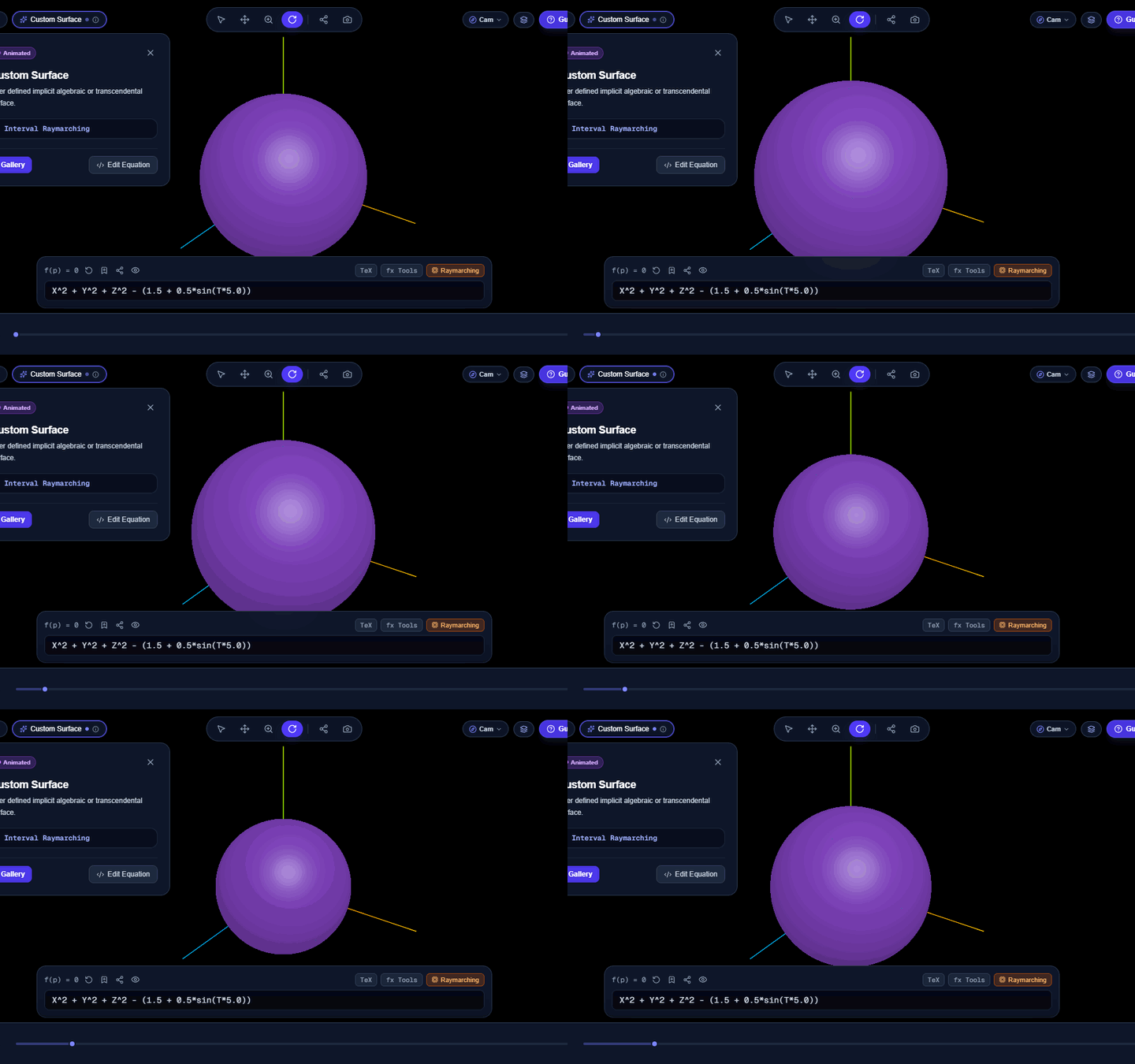
2. $C^1$-Continuous Smooth Minimum (smooth_blend): To create organic fillets where two algebraic surfaces meet, we apply polynomial smooth-minimum blending with radius $k > 0$: $h = \operatorname{clamp}\left(0.5 + \frac{0.5 \cdot (f_2 - f_1)}{k},\, 0.0,\, 1.0\right)$ $F(\mathbf{p}) = \operatorname{mix}(f_2, f_1, h) - k \cdot h \cdot (1.0 - h)$
3. Homotopy Continuation ($\lambda \in [0, 1]$): Enabling Homotopy mode constructs the convex linear combination: $F_\lambda(\mathbf{p}) = (1 - \lambda) f_1(\mathbf{p}) + \lambda f_2(\mathbf{p}) = 0$ Animating $\lambda$ from $0 \to 1$ lets users watch a sphere ($x^2+y^2+z^2-1=0$) continuously deform its genus and bifurcate into the 65-node Barth Sextic!

---

3. Turning Zero-Thickness Surfaces into Watertight 3D Prints (shellThickness)#

Here is a classic trap when exporting an implicit surface $f(x, y, z) = 0$ for 3D printing:

• A surface like the Gyroid ($\sin x \cos y + \sin y \cos z + \sin z \cos x = 0$) or Steiner's Roman Surface is an open, infinitely thin 2D sheet clipped by a bounding sphere or cube.
• If you run Marching Cubes directly on $f(x, y, z) = 0$ inside $[-B, B]^3$, the resulting mesh has zero thickness and open boundary edges where the surface hits the bounding box walls. Every 3D printer slicer rejects open, non-manifold sheets!

To make any algebraic or transcendental surface immediately 3D-printable (src/lib/MeshExporter.ts), we implemented Implicit Offset Shell Thickening (shellThickness $\tau > 0$) combined with Boundary Envelope Capping:

$F_{\text{shell}}(\mathbf{p}) = \max\left( |f(\mathbf{p})| - \tau,\; \|\mathbf{p}\|_{\text{bound}} - B \right) = 0$

• Taking $|f(\mathbf{p})| - \tau = 0$ offsets the zero-isosurface into two parallel sheets at $f(\mathbf{p}) = +\tau$ and $f(\mathbf{p}) = -\tau$, enclosing a solid volume of thickness $2\tau$.
• Intersecting that shell ($\max$) with the bounding volume $\|\mathbf{p}\|_{\text{bound}} - B \le 0$ automatically caps every boundary cross-section, guaranteeing that Marching Cubes extracts a 100% closed, watertight, orientable 2-manifold ready to export as binary STL, vertex-colored OBJ, or GLB (GLTFExporter).